How to Strikethrough in Excel: 10 Steps

Why Use Strikethrough in Excel?

Before jumping into the steps, it helps to know why strikethrough matters. In Excel, strikethrough is a formatting effect, not a delete button. It changes how content looks, but it does not erase the underlying value. That makes it useful for keeping a record of completed tasks, old prices, discontinued products, revised numbers, or items you want to keep for reference without treating them as current.

Think of it as Excel’s polite way of saying, “We’re not using this anymore, but let’s not pretend it never existed.” That’s incredibly handy when you need transparency, version history, or a visual cue that doesn’t require creating an extra column full of awkward labels like “done-ish” or “ignore this one.”

How to Strikethrough in Excel in 10 Steps

Step 1: Select the Cell, Range, or Text You Want to Format

Start by selecting what you want to cross out. This could be one cell, a whole range, or just a few characters inside a cell. If you’re formatting an entire entry, click the cell once. If you want to format several items at the same time, click and drag across a range or use Ctrl on Windows or Command on Mac to select non-adjacent cells.

This sounds obvious, but it matters. Excel only applies strikethrough to what you’ve selected. If you skip this part or accidentally select the wrong range, you may end up crossing out half your list and questioning your life choices before lunch.

Step 2: Use the Fastest Windows Shortcut

If you use Excel on Windows, the quickest way to apply strikethrough is the keyboard shortcut Ctrl + 5. Select the cell or range, press the shortcut once, and Excel applies the line-through effect instantly. Press the same shortcut again and Excel removes it. In other words, it toggles the formatting on and off.

This is the best method when speed matters. It’s perfect for cleaning up checklists, marking completed tasks, or updating a spreadsheet on the fly while pretending you absolutely planned to be this efficient all along. If you work in Excel every day, this shortcut is worth memorizing because it saves more time than you’d think.

Step 3: Use the Mac Shortcut

If you’re on a Mac, the shortcut is Shift + Command + X. Just like on Windows, it works as a toggle. Select the cell, press the shortcut once to apply strikethrough, and press it again to remove it.

Mac users sometimes get stuck because many Excel tips online lean heavily toward Windows. Thankfully, this one is simple. Once you know it, you can move through a worksheet quickly without opening extra menus. It’s especially useful when you’re editing a content plan, sales tracker, or school schedule and want a fast visual signal that something is complete.

Step 4: Open the Format Cells Dialog from the Ribbon

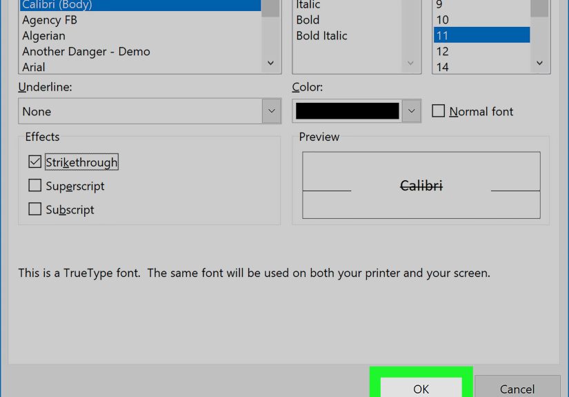
If shortcuts are not your thing, Excel has a menu-based method that works beautifully. Select the cells you want, go to the Home tab, then find the Font group. Click the small dialog launcher arrow in that section to open Format Cells. In the Font tab, check the box for Strikethrough, then click OK.

This method is great for people who prefer to see the setting before applying it. It’s also helpful if you’re already changing other font effects, like bold, italics, color, or size. If the keyboard shortcut is the espresso shot, the Format Cells route is the sit-down coffee. Same result, slightly calmer journey.

Step 5: Open Format Cells with a Shortcut for More Control

There’s also a hybrid approach: open the Format Cells box with a shortcut, then choose strikethrough there. On Windows, use Ctrl + 1. On Mac, Excel supports Command + 1 for the Format Cells dialog. Once the dialog opens, go to the Font tab, check Strikethrough, and confirm.

This approach is ideal when you want more control than the one-tap shortcut gives you. For example, maybe you want to apply strikethrough and also adjust font size, switch colors, or review whether the cell already has mixed formatting. It’s a neat middle ground between fast and precise.

Step 6: Apply Strikethrough to Only Part of the Text in a Cell

Sometimes you don’t want to cross out the whole cell. Maybe the cell says Draft approved on Tuesday, and you only want to strike through the word Draft. In that case, double-click the cell to enter edit mode, highlight only the text you want to format, and then apply strikethrough using the shortcut or the Format Cells method.

You can also work from the formula bar if that feels easier. This is a surprisingly useful trick for notes, product descriptions, version labels, or any worksheet where one cell contains more than one idea. Partial strikethrough is subtle, but when used well, it makes your spreadsheet feel far more polished.

Step 7: Add Strikethrough to the Quick Access Toolbar

If you use strikethrough often, add it to the Quick Access Toolbar. Right-click the toolbar or ribbon, choose the customization option, change the command list to All Commands, find Strikethrough, and add it. Once it’s there, you’ll have a one-click button ready at the top of Excel.

This is a smart setup move for people who live in spreadsheets all day. Finance teams, operations managers, editors, teachers, and project coordinators can all benefit from removing a few extra clicks. It also helps if you’re training other people on a shared workflow, because a visible button is easier to spot than a shortcut buried in memory.

Step 8: Use Strikethrough in Excel for the Web

Yes, you can use strikethrough in Excel for the web too. Select the cells, go to the Home tab, and choose Strikethrough in the Font group. That means you don’t need the desktop app just to cross something out.

This is helpful when you’re editing a shared workbook in a browser, collaborating with a team, or working on a device where the desktop app isn’t available. It keeps the formatting consistent across versions and makes browser-based Excel much more practical for real work. So yes, the web version can absolutely handle this job. No dramatic sighs necessary.

Step 9: Use Conditional Formatting for Automatic Strikethrough

If you want Excel to apply strikethrough automatically, conditional formatting is your friend. Let’s say column A contains tasks and column B contains status values like Done. Select the task cells in column A, go to Home > Conditional Formatting > New Rule, choose Use a formula to determine which cells to format, and enter a formula like =B2="Done". Then click Format, check Strikethrough, and save the rule.

Now Excel applies the formatting automatically whenever the condition is true. This is fantastic for to-do lists, workflow trackers, editorial calendars, issue logs, and assignment planners. It turns strikethrough from a manual formatting trick into a living part of your system. In plain English: Excel does the crossing out for you, and you get to look suspiciously organized.

Step 10: Automate Strikethrough with VBA

If you use macros, VBA can apply strikethrough programmatically. The key property is Font.Strikethrough, which can be set to True or False. That means you can build a button, macro, or automated process that crosses out cells based on your own logic.

This step is best for advanced users, but it’s useful in dashboards, bulk updates, or custom workbook tools. If you manage recurring spreadsheets for clients or teams, VBA can save serious time. Just remember: with great automation comes great responsibility, and occasionally a worksheet that does exactly what you told it to do instead of what you meant.

Best Practices for Using Strikethrough in Excel

Strikethrough works best when it communicates status clearly. Use it for completed, canceled, obsolete, or replaced items. Avoid using it for active items or as a decorative effect. A spreadsheet should not look like it lost an argument with a red pen.

It also helps to stay consistent. If strikethrough means “completed” in one sheet, don’t let it mean “needs review” in another. Pairing it with a status column, color fill, checkbox, or date can make your workbook even easier to interpret.

If strikethrough refuses to go away, check whether it came from conditional formatting rather than normal font formatting. Clearing the font effect alone won’t remove a rule that keeps reapplying it. Likewise, if only part of a cell is crossed out, the cell may have mixed formatting, which can be edited by selecting the specific text in the cell or formula bar.

Common Use Cases for Strikethrough in Excel

• Task lists: Cross out completed action items without deleting them.
• Budgets: Mark removed expenses while keeping a record.
• Inventory sheets: Identify discontinued or sold-out items.
• Editorial calendars: Show published or canceled topics clearly.
• Project trackers: Visually separate completed milestones from active ones.
• Shopping or moving lists: Keep progress visible at a glance.

The beauty of strikethrough is that it gives your data context without deleting history. In spreadsheet land, that is a small miracle.

Experiences With Using Strikethrough in Excel in Real Life

I’ve seen people underestimate this feature until they use it in a real worksheet. Then it becomes one of those tiny Excel skills that quietly improves everything. A simple strikethrough can change a cluttered list into something that feels organized, current, and easy to scan.

One of the most relatable examples is a task tracker. Imagine a weekly operations sheet with twenty or thirty action items. If completed tasks are simply left alone, the list starts to feel chaotic because every line looks equally important. The moment you use strikethrough, the finished work fades into the background without disappearing. That matters. Teams can still see what got done, but their eyes naturally move toward what still needs attention.

The same thing happens with editorial calendars. Content teams often brainstorm far more headlines than they actually publish. Some are approved, some are postponed, and some are dropped because the angle changes. Deleting rejected ideas sounds clean, but it can backfire when someone asks, “Didn’t we already discuss that topic?” A strikethrough keeps the history visible without letting outdated ideas compete with the active plan.

Budget sheets are another great example. Let’s say you’re planning an event and one vendor quote gets replaced with a better one. If you delete the original number, you lose context. If you leave it untouched, people may mistake it for the current price. Strikethrough solves that instantly. The old value stays visible for comparison, but nobody confuses it with the final decision.

Even personal spreadsheets benefit from it. Grocery lists, moving checklists, reading logs, home renovation plans, and holiday prep sheets all become easier to manage when completed items are crossed out instead of erased. It creates momentum. There’s something weirdly satisfying about watching a list fill with neat little lines, as if Excel itself is giving you a quiet round of applause.

What I like most is that strikethrough works for both casual users and spreadsheet power users. Beginners can use a quick shortcut and feel instantly more capable. Advanced users can build it into conditional formatting rules, checkbox systems, or macros. Same effect, different skill level, zero drama.

So yes, learning how to strikethrough in Excel may sound small. But in practice, it’s one of those features that makes a workbook feel smarter, cleaner, and more human. And for a formatting option that is literally just a line through text, that’s pretty impressive.

Conclusion

If you’ve ever wondered how to strikethrough in Excel, the good news is that you have plenty of options. You can use a keyboard shortcut, open the Format Cells dialog, apply it to just part of a cell, add it to the Quick Access Toolbar, use it in Excel for the web, or automate it with conditional formatting and VBA. The best method depends on how often you use the feature and how much control you want.

For most people, the shortcut is the easiest win. For teams and recurring workflows, conditional formatting is the real superstar. Either way, once you start using strikethrough intentionally, your spreadsheets become easier to read and much easier to manage. That’s not bad for one simple line.

SEO Tags